 However, in a business environment that is constantly changing, the use of fixed
quantities can easily result in excess inventory, due to a tendency to over-react to worst-case scenarios,
and planning for the inevitable 'flood' that never comes.
(if you are not using a NETSCAPE-compatible browser, this page may appear poorly formatted)
Table of Contents
Since the 1970's the use of minicomputers, and more recently PC-based networks, have enabled manufacturing
companies to manage their inventory by use of a Material Requirements Planning process, otherwise
commonly known as 'M.R.P.'. Individual requirements for components are derived from bills of material
and the current production plan, so that purchase orders for these components can be generated to maintain
inventory levels above a minimum level, while at the same time considering the various component purchasing
lead times, assembly processing times, economic order quanitities, and so forth. Still, the M.R.P.
process itself is only as good as the production plan, where constant changes to the plan 'inside lead
time' can easily forfeit any benefits derived from a well-designed M.R.P. system. Sudden changes to the
production plan, due to improper forecasting methods, can cause inventory levels
to be unpredictably increased, or can cause sudden shortages that inevitably lead to production line-stops,
often resulting in 'crash buy' programs and expensive expediting and rescheduling. Alternately, to make
up for this front-ended problem, companies will frequently increase their minimum 'safety stock' levels
for process-critical components. Whenever such critical components are expensive, the company ends up with
too much of its assets tied up in inventory, restricting its ability to react to changing markets, and/or
remain profitable in an environment of heavy market competition.
M.R.P. typically relies on STATIC quantities to perform its analysis, and does not inherently provide
any performance feedback to measure production plan accuracy, on-time delivery performance, or the
effect of frequent production plan changes, especially those changes 'inside lead time' that affect
high dollar components.
 However, in a business environment that is constantly changing, the use of fixed
quantities can easily result in excess inventory, due to a tendency to over-react to worst-case scenarios,
and planning for the inevitable 'flood' that never comes.
Such is the result of 'static analysis' of a dynamic system. The tendency here is to see the highest
and lowest values only, and to consider this to be the 'normal range' of values, then plan around these values
by keeping inventory levels excessively high to avoid shortages, or increasing order lead times to a length
of time that more closely approaches a 'build to order' scenario, even when finished goods are typically in
stock when the orders are placed. There are, of course, many contributing factors to these conditions. The
greatest single contributor, though, is the 'static analysis' performed on the dynamic system. The solution,
therefore, is to perform a 'dynamic analysis' on the demand forecast, production plan, and inventory; and one
of the most effective methods of 'dynamic analysis' is Bandwidth Management.
Material Requirements Planning, or M.R.P., is usually implemented by a Discrete
system that operates on individual components, with fixed parameters. A system that uses
Bandwidth Management, however, deals with non-linear "Dynamic" parameters.
When properly implemented, an existing Discrete M.R.P. system can be used to implement
Bandwidth Management, though periodic adjustments would have to be made to the various
static parameters to ensure optimum results. Additionally, a way to monitor Performance
to Plan is needed, to detect potential problem conditions before they become actual
problems. S.F.T. Inc. has provided the Demand Planning Tool for
just this purpose.
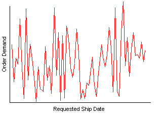
By nature, it is impossible to accurately predict the demand fluctuations placed on a
company by its customers. Normal methods of forecasting demand can seem very accurate,
using various regression techniques, complex exponential smoothing models, and so on.
However, when you apply even the best historically-derived forecast, using the best of
regression models, any one sudden and unexpected change in demand can throw the entire
forecast out of balance, and potentially cause a series of "reactions" throughout
every directly and indirectly affected level of a company, all the way down to the raw stock
and finished goods inventories. Normally, company management makes up for this potential
problem by maintaining high inventory levels, or by establishing long customer order
lead-time requirements, resulting in poor customer satisfaction, increased overhead
costs, and ultimately, reduced revenue.
![]() Normal Distribution Curve
Normal Distribution Curve
 By calculating the Standard Deviation to the mean for the historic data, it is
possible to choose a Z Factor which provides a Confidence Interval that
allows for a balance between low inventory levels, and high customer delivery
performance. The use of Bandwidth Management therefore assumes that the
customer demand will normally fluctuate within such limits of the Normal Distrubution
Curve, based upon the Standard Deviation, and a desired Confidence Interval.
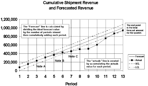
This calculation forms the Upper and Lower Control Limits, between which the measured
parameter (customer order rate, backlog, lead time, inventory levels, and so on) can
fluctuate without requiring any corrective action. The standard deviation multiplied
by the 'Z' factor, then added to and subtracted from the median value, forms the
Control Band, within which normal values of the measured parameter are expected
to fluctuate. Actual values that fall within the control band are therefore considered to be
"normal", and therefore require no corrective actions. Only those values that fall
either above or below the Control Band require analysis, and possible corrective
action. Alternately, the control band can be calculated based on a pre-defined minimum or
maximum control limit, to which twice the standard deviation times the 'Z' factor is added to
(or subtracted from) the minimum (or maximum) value to form the control band. Therefore, by
defining a normal control band based on statistically derived parameters, it is possible to
significantly reduce the amount of work load for analysis and corrective action regarding nearly
any established parameter, whether a demand forecast, inventory levels, customer order backlog,
safety stock, or lead time.
Let us define a company, known as 'Company A', that sells an average of 10,000 units of
its 'Product B' line per year. Over the last 3 years, by linear regression, they show
a relatively constant rate of sales with this product line. However, on a month-to-month
analysis, they show a fluctuation between 200 and 2300 units sold within a month, and
on a week-to-week basis, the sales range from zero to 1900 units in a single week, during
the last 3 years of history.
The management of 'Company A' is concerned that its inventory levels are too high, although
they have kept them high due to constant fluctuations in the production schedule for its
'Product B' line, as the Marketing department has been constantly adjusting the demand
forecast that Operations uses to generate its master schedule. Consequently, without high
inventories, the sudden demand changes would result in material shortages, line stops,
and so on. Further, a large segment of the work force is continuously being laid off and
re-hired based on the current needs, and often work 10 or more hours of overtime during
the peak periods.
Therefore, 'Company A' decides to apply Bandwidth Management to their demand
forecasting process, and predicts a monthly sales rate of 833 units, with a bandwidth (based
on the standard deviation and an 85% confidence interval) of +/- 1870 units. To account
for the worst-case demand fluctuation, they maintain an average of 1870 units in finished
goods, so that they can provide the 'off the shelf delivery' that their customers demand,
under the 'worst case' conditions as defined by the bandwidth. Then, they schedule their
production so that a constant 833 units is produced every month. The result of this gives
them approximately 23 inventory turns on finished goods for this product, which is outstanding
considering that they are providing 'off of the shelf' delivery to their customers.
Since Operations now has a consistent build schedule, they are able to reduce their raw stock
inventories and negotiate better prices with their suppliers on long-term delivery
contracts. And, since the raw stock deliveries are not being constantly re-scheduled,
their suppliers are more willing to work with them on quality issues and on-time delivery
problems from their end as well. And, the shop floor work force is no longer subject to
constant layoff and re-hire situations, which improves morale and retains more quality
personnel.
The overall effect on 'Company A's business has been positive. They have reduced their
inventories, cut 'hidden' costs due to constant demand changes, improved their ability
to react to changes by absorbing the affect over a longer period of time, and improved
the morale and quality of the shop floor work force by providing them with more stable
employment, and without excessive overtime.
One excellent way to demonstrate the effectiveness of Bandwidth Management can be found
 in the world of power generation, in a typical steam plant that is designed to respond
to varying loads without having a large 'inventory' of water, such as on board a ship.
In such a steam plant, you need to maintain water level in the boiler within a specific
range. If the level is too high, liquid water will end up in the steam pipe and damage
the turbines. If the level is too low, you uncover the tubes (whether it is a fire-tube,
a water-tube, or a nuclear 'heat exchanger' boiler) and risk damaging the boiler itself.
In addition to this, you have the 'varying demand' on the boiler, as represented by the
propulsion system on board a ship, or a widely varying electrical load in a commercial
power generating plant. As the demand for steam increases, you must pump water into the
boiler at a higher rate than before to maintain the level. Further, the level indicators
will show a higher level at higher steam rates due to the increased boiling, as when a pot
on the stove boils up and spills over the edges, without having to increase the amount of
water in the pot.
Thus, we define our analogy of a 'manufacturing system' as applied to a boiler. You have
raw materials being applied (in this case, water). The inventory parameter we are
controlling is the amount of water in our boiler (the warehouse). The production plan
(the burner or nuclear reactor) is designed to quickly respond to changes in demand, by
rapidly changing the production plan (burn rate) to match forecasted demand (throttle position)
and actual demand (steam flow rate). And, we want to avoid cyclically stressing the equipment
to prevent damage, and therefore make gradual changes to our water flow and steam production
rate.
In a boiler control system, there are several different approaches that can meet the requirements
needed to accomplish the desired task. First, you can use a "bi-stable" method, which starts
adding water when level drops to a specific point, then stops adding water when it rises to a
maximum point. This is like a 'safety stock' inventory model. To work properly, it requires a
large amount of inventory, short lead times on request for new material, but has very high
flexibility on demand changes. Unfortunately, suppliers rarely allow orders to be made within
such a short lead time, so the safety stock levels end up being high enough to allow for the
worst-case lead time. In short, you have too much inventory with this method.
A slightly better method for inventory control involves a continuous flow and a throttle valve.
The throttle valve adjusts the amount of water (raw materials) that are continously being added
to our boiler, responding only to changes in level. As level gets too low, the throttle control
opens the throttle to allow more water to enter the boiler. However, if the water level
drops faster than the throttle's ability to open to match the demand, the level will drop too low.
Conversely, if the water level shoots up faster than the throttle's ability to shut, the level will
rise too high. Therefore, to compensate for delays in changing the supply rate (purchase and
reschedule lead-times) the inventory level is increased to match worst-case supply lead time response,
in a 'just in case' scenario.
However, if 'bandwidth management' were applied to our boiler, it would work something like this:
The boiler is built to house a minimum amount of water, based on its maximum ability to produce steam
and the amount of manufacturing surface required to produce the designed capacity of steam. The steam
flow (either booked orders or shipments) is measured and compared to the the feed-water flow rate
(supply of raw materials). In addition, the "ideal level" in the boiler is calculated based on the
average steam flow rate (shipments or booked orders) over a period of time that is greater than the
ability of the throttle valve (purchase orders and re-schedules) to respond to changes in demand.
A bandwidth, equal to a multiple of the statistical standard deviation of demand changes over the same
period in time as the demand average, is applied on both sides of the ideal level, so that changes in
level on either side of the bandwidth cause no change in throttle position (raw material supply).
However, if an 'error signal' between supply and demand indicate a change in demand larger than the
expected changes inside bandwidth, the throttle valve position changes, to match the 'total error'
signal, and maintain inventory level within the control band by anticipating the need before level
drops too low. Thus, the danger of 'over-compensation' is eliminated, as well as eliminating the
danger that the ability to change supply will not meet the ability to change demand.
In order to properly apply Bandwidth Management principles to your business, it
is necessary to have adequate time-phased historic data available that can be analyzed
for average, linear regression, and standard deviation information. Alternately, other
models can be applied to obtain slightly more accurate median values about which
the control bands are assigned, but for all practical purposes an average or linear
regression line provides for an adequate (and easily generated) set of control bands.
Typically, you will need at least 2 years' worth of historic data, with time-phased data
summarized either by week or by day, in order to obtain a meaningful standard deviation.
Data which is summarized by a time period greater than one week increases the amount of
time needed to detect errors properly, and causes too many "spurious" errors (actual values
that fall outside of the established control limits), since the standard deviation is too
small to account for normal day to day deviation. On the other hand, information that is
summarized by a time period less than one day causes the amount of time to generate the
necessary calculations to increase unnecessarily, and may result in control limits that are
too large to yield adequate results.
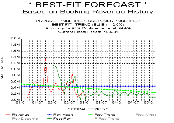
Because of the impact that an Accurate Demand Forecast
can have on the total success of a business, a Demand Forecast will be used for this
example on implementing Bandwidth Management. The numbers used here are from an actual
company which is experiencing a downward trend in business, forcing them to re-examine various
aspects of the business, including forecast accuracy. The graphs shown below were generated
using the Demand Planning Tool's Demand Analysis and Forecast modules.
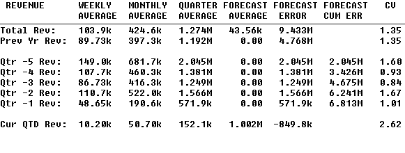
Once we have generated an accurate forecast, we can begin measuring performance to this forecast.
As orders are placed, they should fall within the control band, based on the specified confidence
interval and standard deviation for the historic data. This chart below indicates some of the
statistics that we can obtain from the historic data, historic forecast, and current forecast for
the product family that we are analyzing. As you can see, actual bookings to forecast has been
rather poor. As it turns out, this company had been measuring their performance to shipments,
not to bookings. But, in the case of this product family, shipment rescheduling artificially added
its own component to the process, which threw off the forecast analysis, leading people to inaccurately
believe that their forecast was good. However, from the customer's perspective, the resulting
long lead times between order placement and order delivery created a situation of poor customer
satisfaction, and a tendency to make large "bulk" orders, resulting in artificial seasonality.
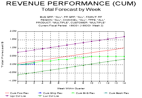
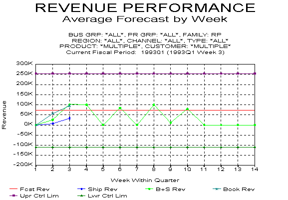
The following chart below shows our current position cumulative booking position within the current
fiscal quarter, and the upper and lower control limits that were statistically derived from the historic
booking revenue data, and applied to the current quarter's forecast, averaged per week.
One additional benefit of Bandwidth Management is the exclusion of all but the "problem items" from the list
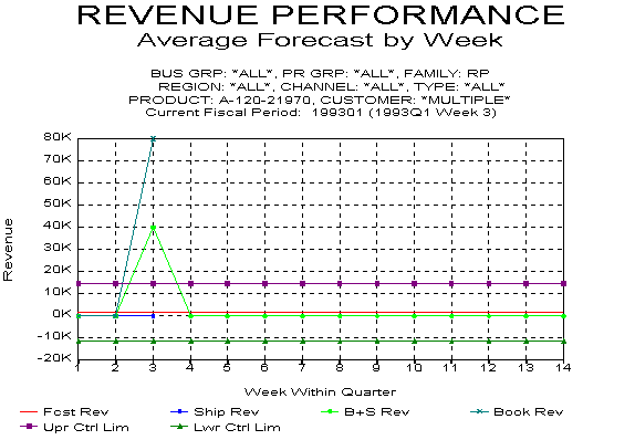
of product and/or customer data that needs to be analyzed. In the case above, only a single product within the
entire product family showed any sign of problem; all of the others fell within the established control limits.
Therefore, instead of managing 17 individual products, only one needed to be checked. And, if the problem had shown
up at the product family level, or the product group level, a further analysis would reveal the actual cause of the
problem. So, analysis at the top level (business group, product group, or product family) can be quickly
accomplished by senior managers, and the more detail-oriented work (product-level analysis) can be performed by
more junior personnel. Still, the actual problems can be detected programatically; any parameter which violates a
control limit could generate an "exception signal", and the resulting exception could be reported to the appropriate
person on a weekly, or even daily, basis. Such "exception reporting" frees up personnel to do other, more important
activities, such as troubleshooting the causes for the various exceptions, and making appropriate corrective actions,
rather than spending all of their time immersed in detail, trying to find out whether a problem exists in the first
place.
The Demand Planning Tool, a product of S.F.T., Inc., is a combined effort of over 5 years of
development work, and is designed primarily to allow the user to quickly generate a more accurate forecast, maintain
this forecast along with a long-term business plan, and perform daily or weekly Demand Analysis to measure
current performance (actual data) to the forecast. It contains a number of screens, graphs, and reports to make this
process as easy and fast as possible. The majority of the graphs and screens shown above were generated using the
Demand Planning Tool, and were specifically designed with Bandwidth Management in mind.
Once an accurate forecast has been generated, a vast majority of the customer orders will fall within the statistically
based control parameters. To facilitate easy detection of potential problem conditions, the Demand Planning Tool has a
screen to perform 'Exception Planning', which generates a pareto listing of demand exceptions, using one of 6 different
analyses, in "reverse dollar" order (so that the items with the highest dollar impact will appear at the top of the list).
In this way, any items that fall outside of the normal control limits will show up, and the pareto order allows the highest
impact items to be dealt with first. Further, since only a fraction of the total number of items are being dealt with,
even at the customer and product level, far more real analysis work can be done with fewer man-hours. This, in turn,
saves money, and the long term benefits can easily offset the cost of the Demand Planning Tool within a
relatively short period of time.
©1995,1996 by Stewart~Frazier Tools, Inc. - all rights reserved
Last Update: 10/02/96